Whenever you’re working with massive datasets, it’s helpful to know the best way to filter in Google Sheets.
There are two methods to do that. You need to use filter views within the Google Sheets menu, which helps you to customise particular methods to filter the information within the sheet that you would be able to reuse. A extra dynamic technique to filter knowledge in Google Sheets is utilizing the FILTER operate.
On this article, you’ll learn to use each strategies.

Create a Filter View in Google Sheets
On this technique, you’ll learn to apply a filter that can present you solely knowledge from a big dataset that you just need to see. This filter view will cover all different knowledge. You can too mix filter parameters for extra superior filter views as effectively.
The right way to Create a Filter View
For example, think about you've got a set of knowledge that features product purchases made by clients. The information consists of names, addresses, emails, cellphone numbers, and extra.
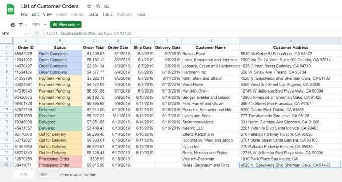
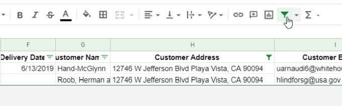
For this instance, let’s say you need to see solely clients from Playa Vista, CA, and solely clients who've a “.gov” e-mail handle.
1. To create this filter, choose the Create a Filter icon within the menu. This icon seems like a funnel.

2. You’ll see small filter icons seem on the best aspect of every column header. Choose this funnel icon on the prime of the Buyer Tackle area to customise the filter for this area.
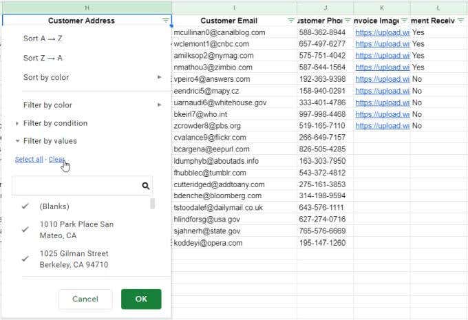
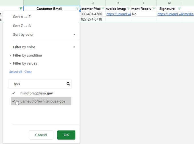
3. This can open a window the place you may customise the filter choices. Choose the arrow to the left of Filter by values. Choose Clear to deselect all entries in that area.
Be aware: This is a vital step as a result of it resets the view from exhibiting all information to exhibiting none. This prepares Excel to use the filter you’re going to create within the subsequent steps.
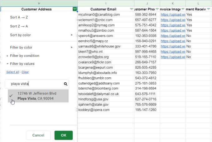
4. Sort the textual content within the area under that you just need to filter the sphere by. On this instance, we’ll use “Playa Vista” and choose the search icon to see solely these information that comprise that textual content. Choose the entire information that present up within the outcomes record. This customizes your filter in order that solely the objects you choose will likely be displayed within the spreadsheet.
4. As soon as you choose the OK button, you’ll see the information in your sheet filtered in order that solely clients from Playa Vista are displayed.
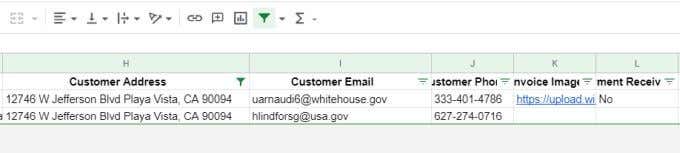
5. To filter on a second area, choose the filter icon on the prime of that area. Repeat the method above to create the filter. Clear all entries, sort the “gov” textual content to filter out any e-mail addresses that don’t comprise “gov,” choose these entries, and choose OK.
Now you’ve personalized your filter in order that solely the information within the dataset you care about are displayed. So that you just don’t need to repeat this course of each time you open the spreadsheet, it’s time to save lots of the filter.
Saving and Viewing Filter Views
Whenever you’re accomplished organising your filter, it can save you it as a filter view that you would be able to allow at any time.
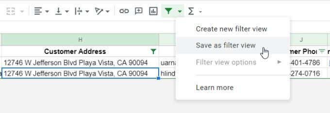
To avoid wasting a filter view, simply choose the dropdown arrow subsequent to the filter icon and choose Save as filter view.
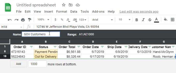
You’ll see a darkish grey area open on the prime of the spreadsheet. This can present you the chosen vary that the filter applies to and the identify of the sphere. Simply choose the sphere subsequent to Identify and sort the identify you’d like to use to that filter.
Simply sort the identify and press Enter.
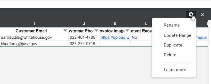
You’ll discover on the best aspect of the grey bar that there’s a gear icon. Choose this icon to see filter choices.
Obtainable choices embody:
- Rename the filter
- Replace the vary that the filter applies to
- Duplicate the filter to replace it with out affecting the unique filter
- Delete the filter
You'll be able to flip off the filter you’ve enabled at any level just by deciding on the filter icon once more.
Be aware that when any filter is enabled, the filter icon will flip inexperienced. Whenever you disable the filters, this icon will flip again to black. This can be a fast technique to see the whole dataset or if any filter has eliminated knowledge from the present view.
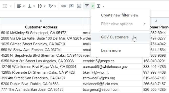
Later, if you wish to re-enable any of the filters you’ve created, simply choose the dropdown arrow subsequent to the filter icon. You’ll see the filters you’ve saved seem within the menu. Simply choose that filter to allow it everytime you like.
This can filter the view once more utilizing the filter settings you’ve configured.
Utilizing the FILTER Operate
One other choice to filter in Google Sheets is utilizing the FILTER operate.
The FILTER operate helps you to filter a dataset based mostly on any variety of situations you select.
Let’s check out utilizing the FILTER operate utilizing the identical Buyer Purchases instance because the final part.
The syntax of the FILTER operate is as follows:
FILTER(vary, condition1, [condition2, …])
Solely the vary and one situation for filtering are required. You'll be able to add as many further situations as you want, however they aren’t required.
The parameters of the FILTER operate are as follows:
- vary: The vary of cells you need to filter
- condition1: The column or rows that you just need to use to filter outcomes
- conditionX: Different columns or rows you’d additionally like to make use of to filter outcomes
Take into account that the vary you employ to your situations must have the identical variety of rows as the whole vary.
For instance, if you wish to create the identical filter as the primary a part of this text, you’d use the next FILTER operate.
=FILTER(F1:J20,SEARCH(“Playa Vista”,H1:H20),SEARCH(“gov”,I1:I20))
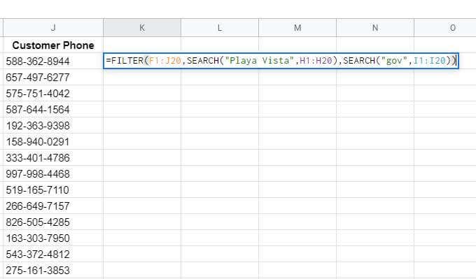
This grabs the rows and columns from the unique desk of knowledge (F1:J20) after which makes use of an embedded SEARCH operate to go looking the handle and e-mail columns for the textual content segments that we’re concerned with.
The SEARCH operate is just wanted if you wish to search for a textual content phase. If you happen to’re extra concerned with a precise match, you may simply use this because the situation assertion as an alternative:
I1:I20=”nmathou3@zimbio.com”
You can too use different conditional operators, like > or < if you wish to filter values higher than or lower than a hard and fast restrict.
When you press Enter, you’ll see the outcomes of the FILTER operate as a outcomes desk.
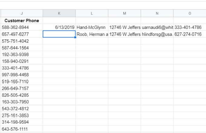
As you may see, solely the columns within the vary you chose within the first parameter of the operate are returned. So it’s vital to put the FILTER operate in a cell the place there’s room (sufficient columns) for the entire outcomes to look.
Utilizing Filters in Google Sheets
Filters in Google Sheets are a really highly effective technique to dig by way of very massive units of knowledge in Google Sheets. The FILTER operate provides you the pliability of maintaining the unique dataset in place however outputting the outcomes elsewhere.
The built-in filter function in Google Sheets helps you to modify the lively dataset view in no matter manner you’re at any given second. It can save you, activate, deactivate, or delete filters nonetheless you want.
Do you've got any fascinating tricks to supply for utilizing filters in Google Sheets? Share these within the feedback part under.
Post a Comment